The simple linear regression is a predictive algorithm that provides a linear relationship between one input (x) and a predicted result (y).

We will take a look at how we can do it by hand and then implement logic in Rust that does exactly this automatically.

Table of Contents

The simple linear regression

Imagine a two-dimensional coordinate system with 2 points. We can connect both points with a straight line and also calculate the formula for that line. That formula has the form of y = mx + b.

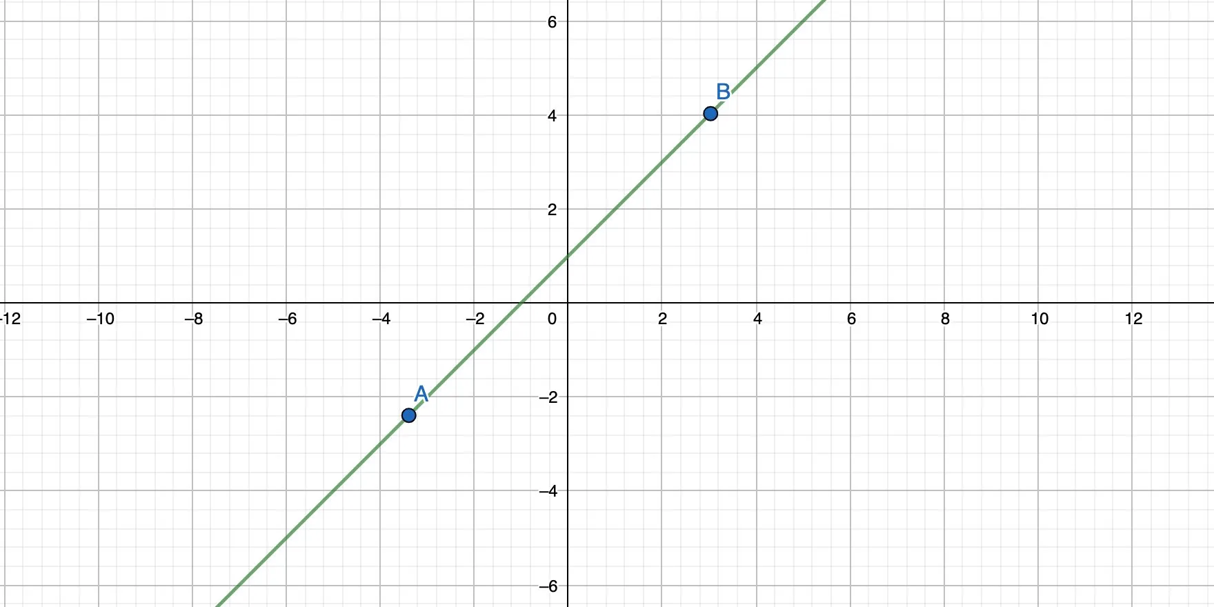
• b is the intercept. It’s the point where the straight line crosses the y-axis.
• m is the slope of the line.
• x is the input.

With only two points, calculating y = mx + b is straightforward and doesn’t take that much time. But now imagine that we have a few more points. Which points should the line actually connect? What would its slope and intercept be?

The simple linear regression solves this problem by finding a line that goes through a cloud of points while minimizing the distance from each point to the line.

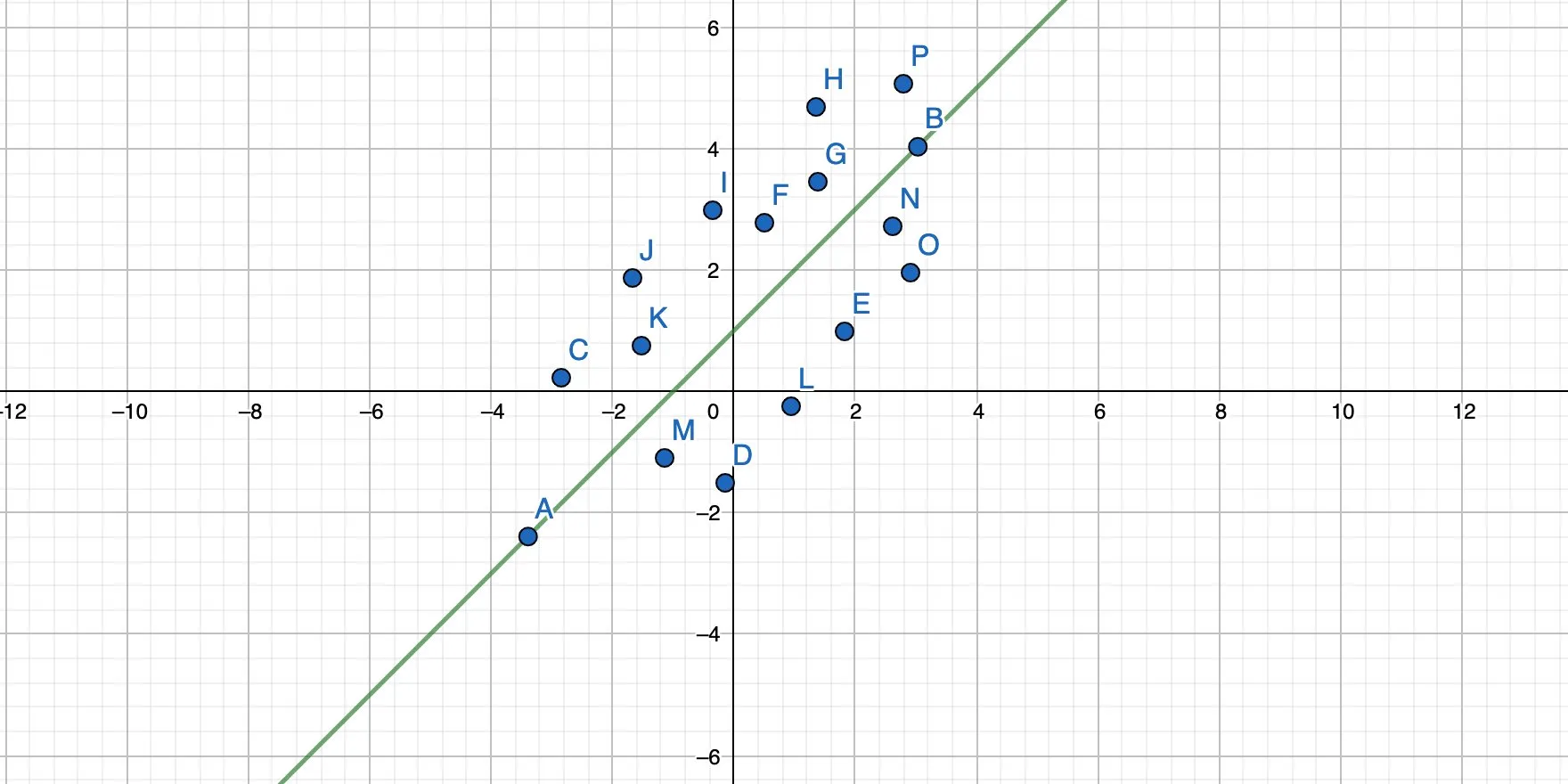
In other words: Find the best possible solution while, most likely, never hitting the exact result. But that result is close enough so that we can work with it.

We basically rotate the straight line until all points have the minimum possible distance to the line, like this:

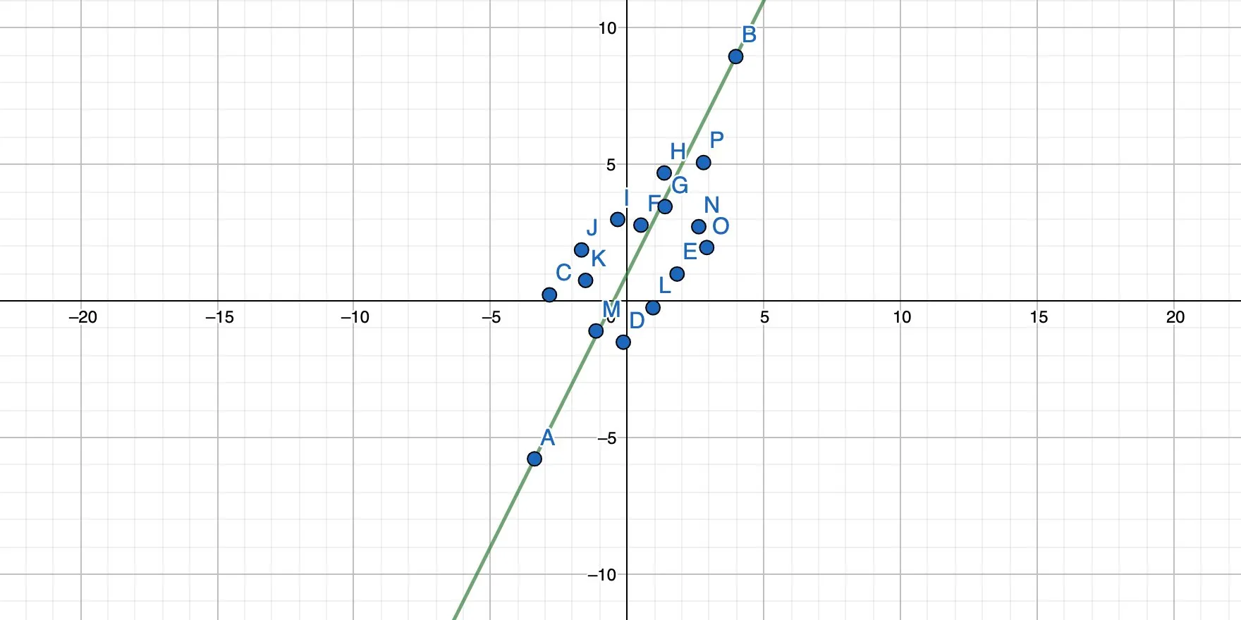
And this:

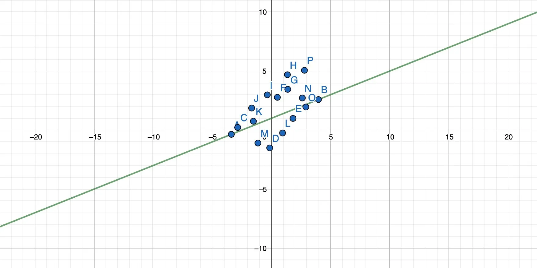
And this:

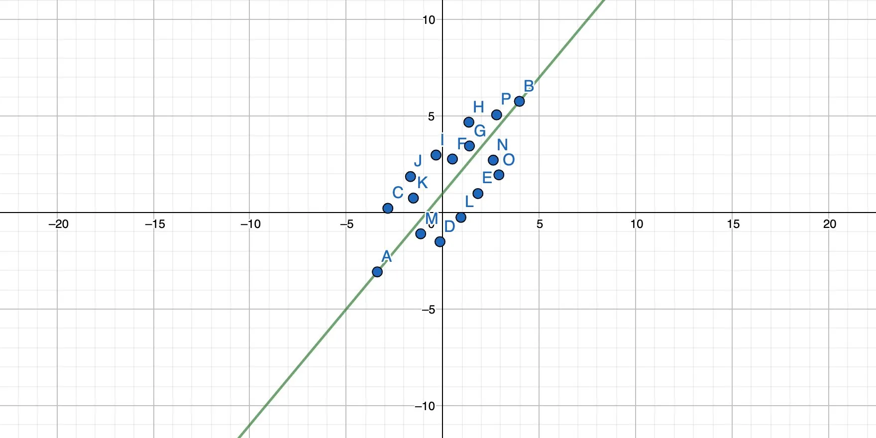
The result is a function that also has the form y = mx + b, and each x passed into this function yields a result of y, which is the prediction for this particular input.

As you might be able to guess already, the simple linear regression is not a fit for all problems. It’s useful when there is a linear relationship between our input x and the outcome y but way less useful when that relationship is not linear. In that case, we are better off using another algorithm.

Some math

We can’t get around math if we want to understand how the simple linear regression works but let’s try to circumvent most mathematical expressions, and only look at what’s really necessary.

To make things easier, we’ll use Excel to look at the math and experience an example scenario. (You can follow along (Google Docs works, too) if you like.)

In this case, we assume that the area (in square meters) of a house directly affects its price. This scenario ignores that there may be more input variables affecting the price, like location, neighborhood, and so on. It’s only very basic, but should be enough for us to understand the simple linear regression and the math associated with it.

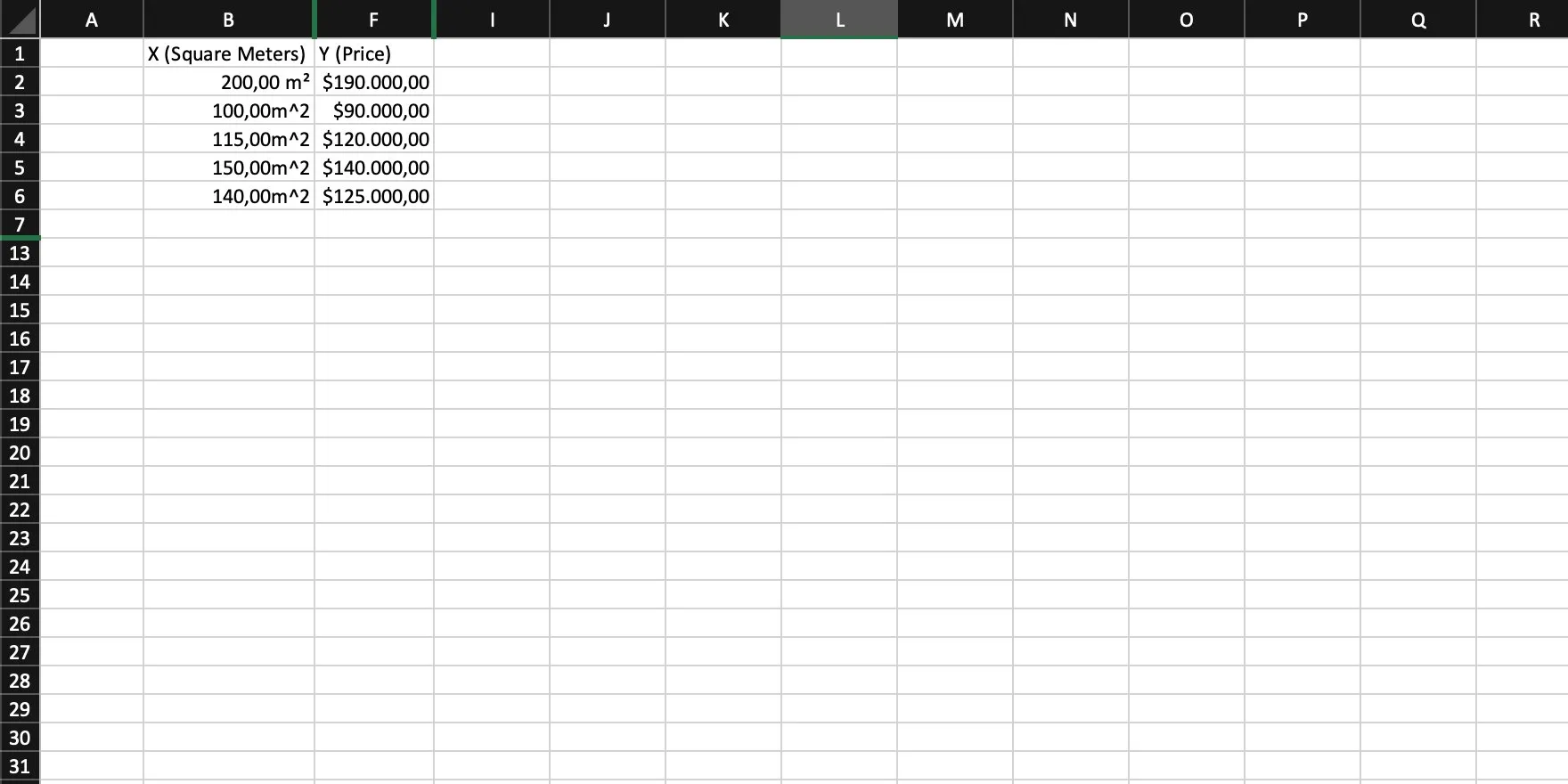
Start

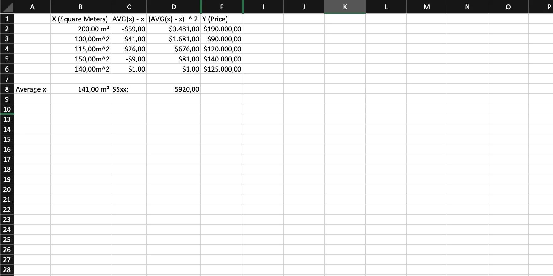
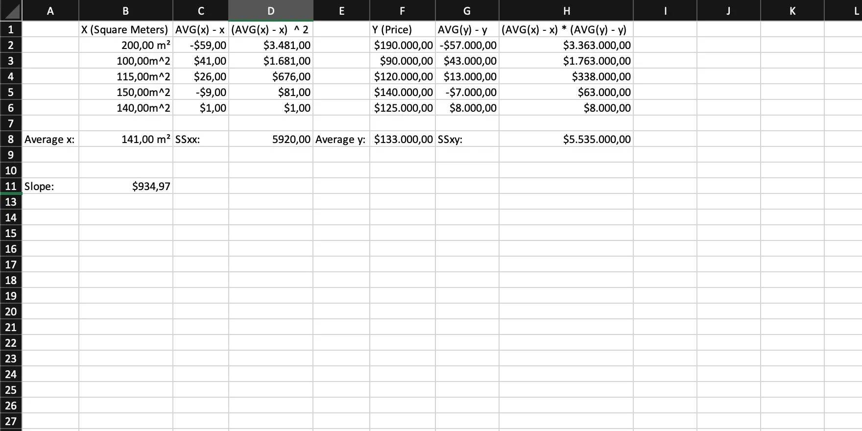
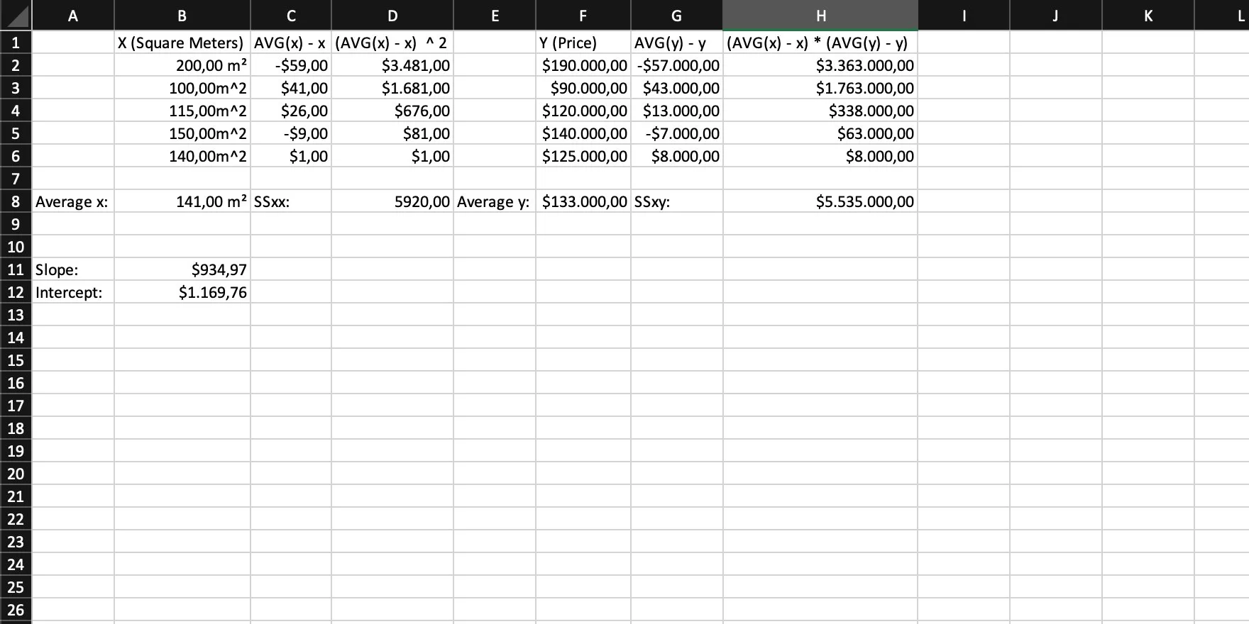
The starting point is a collection of house sales, listed as the area in square meters, and the price each house was sold for.

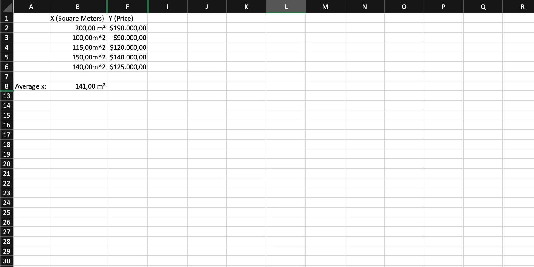
Step 1

Calculate the average of x. We need to sum up all values and then divide that sum by the number of values (or simply use an AVG function).

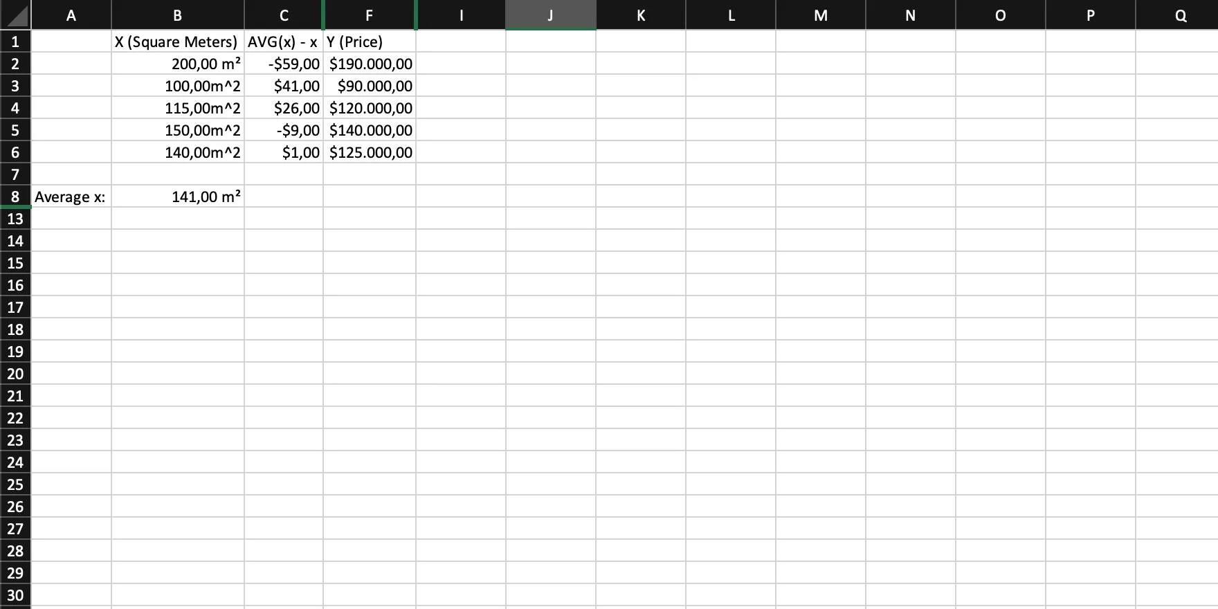
Step 2

We now need the difference of each individual x to the average of x. In other words: For each x, calculate AVG(x) - x.

Step 3

We calculate the variance of x, called SSxx by:

• Squaring the difference of each x to the average of x
• Summing them all up

The variance basically states how far observed values differ from the average.

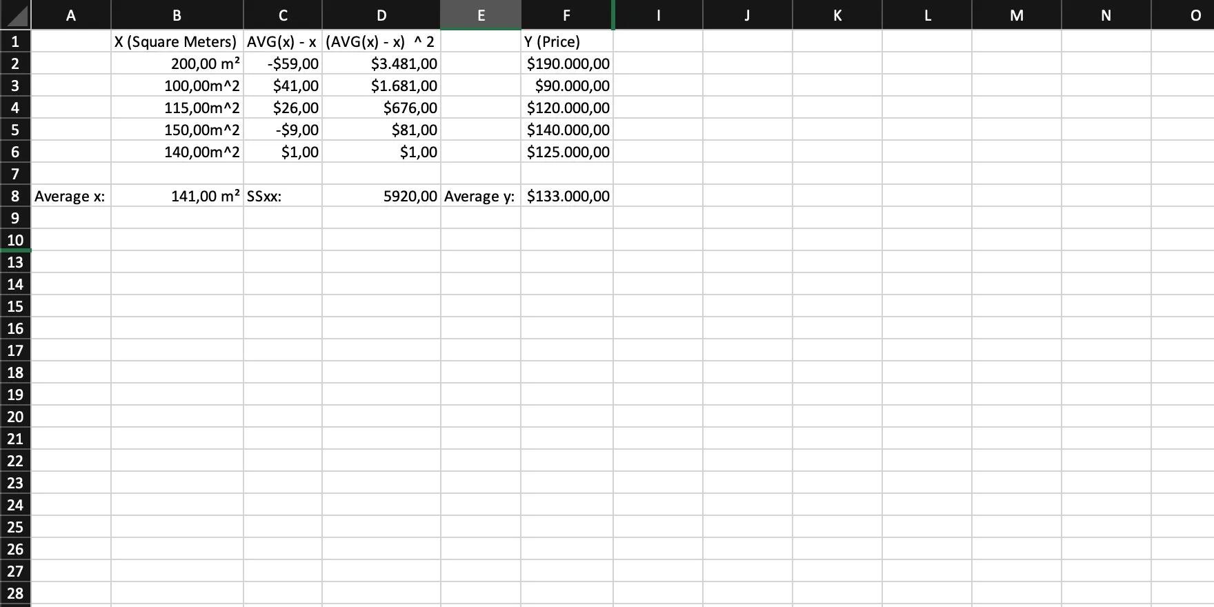
Step 4

Then we need the average of our y. Like we already did for x, we sum them all up and divide that sum by the total amount of values (or use an AVG function).

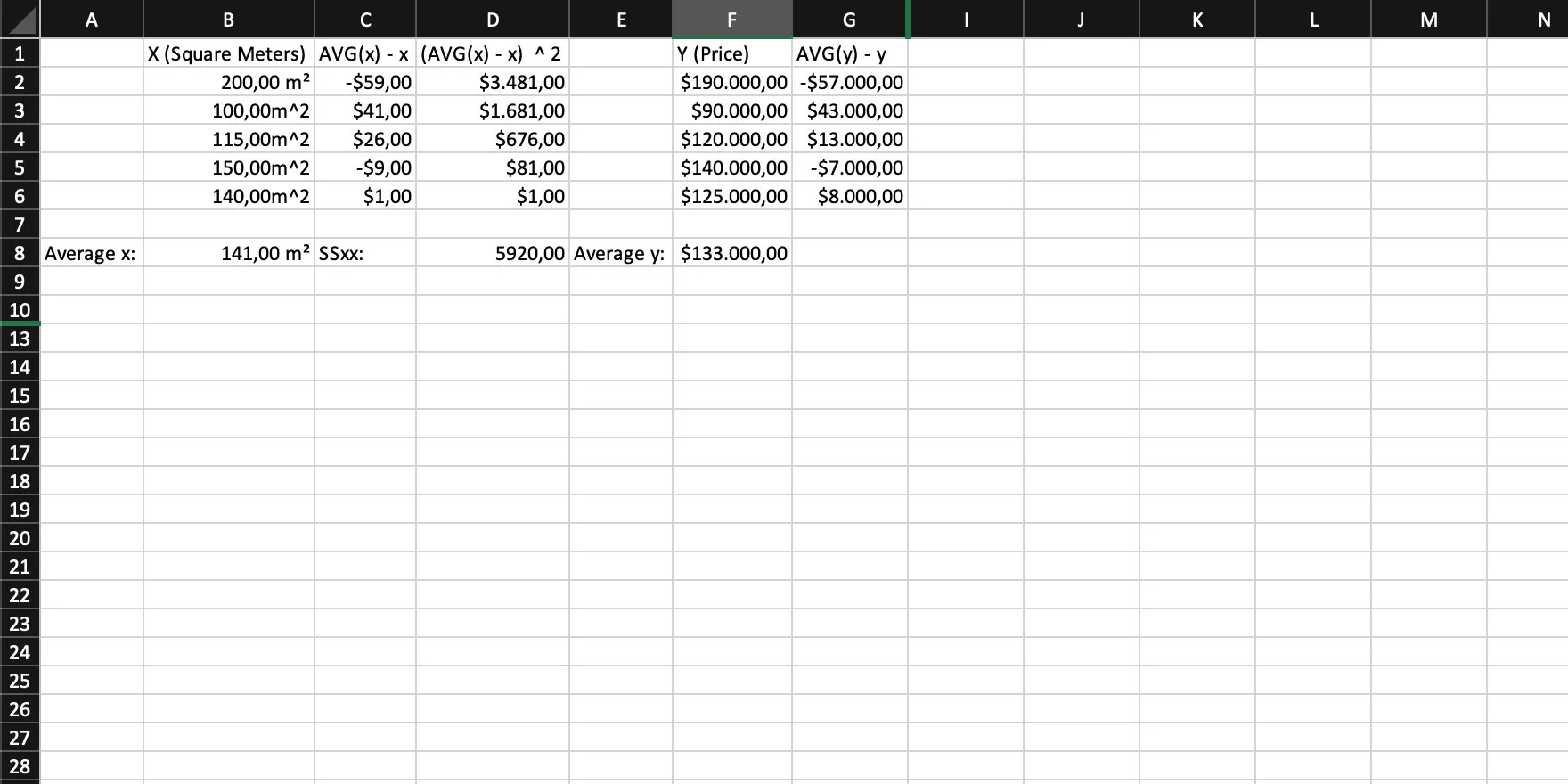
Step 5

We calculate the difference of each y to the average of y. In other words: For each y, we calculate AVG(y) - y (Yes, this is step 2 but for y).

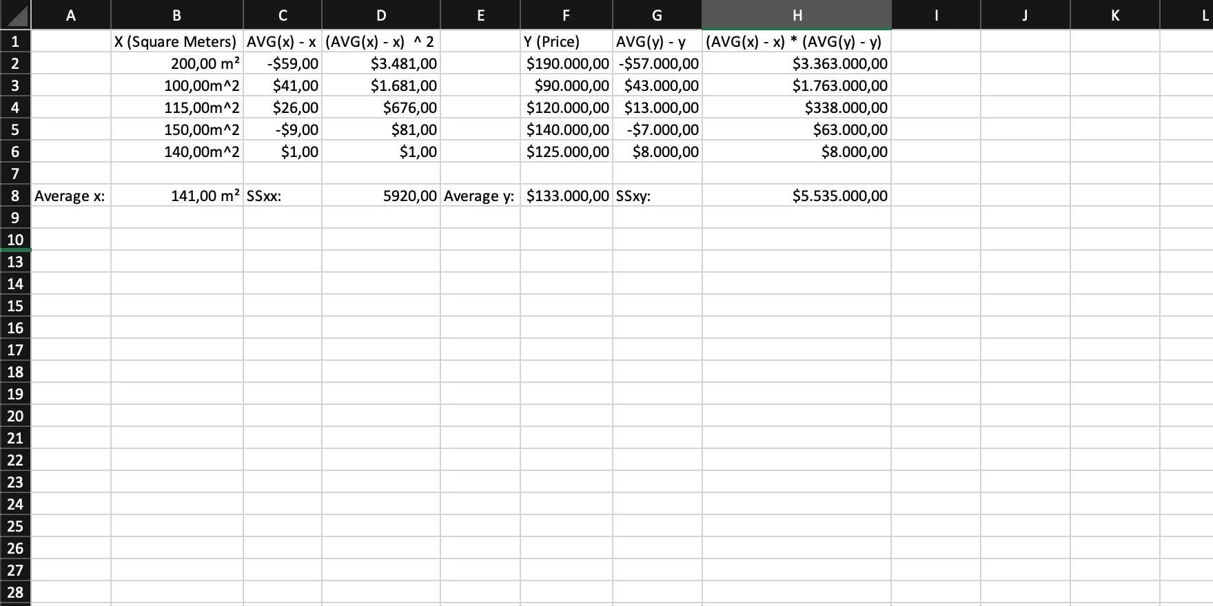
Step 6

Now we multiply the individual differences of x/y by their respective average and sum them up. This is SSxy, the covariance of x and y.

Step 7

Then we calculate the slope, using SSxx and SSxy with the following formula: slope = SSxy / SSxx = m.

Step 8

The last thing to do is to calculate the intercept with the formula: intercept = AVG(y) - slope * AVG(x) = b.

Step 9

We’re done! We can simply put everything together and have our linear function: y = intercept + slope * x = 1169.76 + 934.97 * x.

Implementing the simple linear regression in Rust

Until now, everything we did was based on Excel. But it’s way more fun to implement something in a real programming language, and this language is Rust (of course).

The goal is to create a function that performs our simple linear regression and then returns a struct that has the formula baked into it, so we can easily call a method with different input at any time after “training” our regression to make predictions.

Into the Code

Let’s assume that our input is a vector containing a tuple with two members, our x and y values. In this case, our x stands for the area of the house (in square meters), and our y stands for the price in dollars that house was sold for:

fn main() {
  let vec = vec![
      (200., 190000.),
      (100., 90000.),
      (115., 120000.),
      (150., 140000.),
      (140., 125000.),
    ];
  }

An important next step is to create a linear regression struct that holds both intercept and slope and additionally offers a method that calculates an output y for an input x:

pub struct LinearRegression {
  intercept: f64,
  slope: f64,
}

impl LinearRegression {
  pub fn calculate(&self, x: f64) -> f64 {
      self.intercept + self.slope * x
  }
}

That’s everything we need to perform calculations later. The most important thing, actually training our algorithm, however, is still missing.

Let’s add a static function to our struct that allows us to “train” a new instance of our regression by passing our input to it in the form of a slice containing a tuple, which in return consists of two 64-bit floating point values:

impl LinearRegression {
  pub fn train(input: &[(f64, f64)]) -> Self {

  }

  // rest of the impl...
}

The first step in training our linear regression now is to split our input vector into two separate ones, each containing either the x or the y values:

impl LinearRegression {
  pub fn train(input: &[(f64, f64)]) -> Self {
    let x_list: Vec<f64> = input.iter().map(|pairs| pairs.0).collect();
    let y_list: Vec<f64> = input.iter().map(|pairs| pairs.1).collect();
  }

  // rest of the impl...
}

Based on the first vector, our x values, we can then sum them up and calculate their average. Numeric iterators in Rust thankfully already provide a sum() method, so there’s not that much code to write. For the average, we can divide that sum by the vector’s length:

impl LinearRegression {
  pub fn train(input: &[(f64, f64)]) -> Self {
    // hidden for readability

    let avg_x: f64 = x_list.iter().sum::<f64>() / x_list.len() as f64;

  }

  // rest of the impl...
}

Then we need the difference of each individual x to the overall average of x, and additionally, all these values squared:

impl LinearRegression {
  pub fn train(input: &[(f64, f64)]) -> Self {
    // hidden for readability

    let x_differences_to_average: Vec<f64> = x_list.iter().map(|value| avg_x - value).collect();
    let x_differences_to_average_squared: Vec<f64> = x_differences_to_average
        .iter()
        .map(|value| value.powi(2))
        .collect();
  }

  // rest of the impl...
}

The squared values are the base to calculate SSxx from, which is just their sum:

impl LinearRegression {
  pub fn train(input: &[(f64, f64)]) -> Self {
    // hidden for readability

    let ss_xx: f64 = x_differences_to_average_squared.iter().sum();
  }

  // rest of the impl...
}

Okay, time for a small break. Let’s take a deep breath, recap what we have done until now, and take a look at how our function should now look like:

impl LinearRegression {
  pub fn train(input: &[(f64, f64)]) -> Self {
    let x_list: Vec<f64> = input.iter().map(|pairs| pairs.0).collect();
    let y_list: Vec<f64> = input.iter().map(|pairs| pairs.1).collect();

    let avg_x: f64 = x_list.iter().sum::<f64>() / x_list.len() as f64;

    let x_differences_to_average: Vec<f64> = x_list.iter().map(|value| avg_x - value).collect();
    let x_differences_to_average_squared: Vec<f64> = x_differences_to_average
        .iter()
        .map(|value| value.powi(2))
        .collect();

    let ss_xx: f64 = x_differences_to_average_squared.iter().sum();
  }

  // rest of the impl...
}

Half of the work is now done but handling y is still missing, so let’s get the average of y like this (which is basically the same way we calculated the average of x):

impl LinearRegression {
  pub fn train(input: &[(f64, f64)]) -> Self {
    // hidden for readability

    let avg_y = y_list.iter().sum::<f64>() / y_list.len() as f64;
  }

  // rest of the impl...
}

Like we already did for x, we also need the difference of each y to the average of all of them:

impl LinearRegression {
  pub fn train(input: &[(f64, f64)]) -> Self {
    // hidden for readability

    let y_differences_to_average: Vec<f64> = y_list.iter().map(|value| avg_y - value).collect();
  }

  // rest of the impl...
}

The next step is to multiply each difference of x to the average by the corresponding difference of y to the average. We can use zip() for that and merge both vectors together. The result is one iterator over a tuple of pairs of differences. In this case, we don’t need to worry about zip()’s behavior on iterators of different length as it’s guaranteed that both vectors have the same length (If you’re still wondering: Everything we work with originates from one single slice containing a tuple. As we have only split x and y into separate vectors, it’s guaranteed that they all have the same length):

impl LinearRegression {
  pub fn train(input: &[(f64, f64)]) -> Self {
    // hidden for readability

    let x_and_y_differences_multiplied: Vec<f64> = x_differences_to_average
          .iter()
          .zip(y_differences_to_average.iter())
          .map(|(a, b)| a * b)
          .collect();
  }

  // rest of the impl...
}

Now we can finally calculate SSxy, which is simply the sum of the multiplied differences we have just calculated:

impl LinearRegression {
  pub fn train(input: &[(f64, f64)]) -> Self {
    // hidden for readability

    let ss_xy: f64 = x_and_y_differences_multiplied.iter().sum();
  }

  // rest of the impl...
}

With everything in place, we can finally calculate the slope and the intercept of the straight line going through the cloud of points and then return an instance of our struct holding the regression:

impl LinearRegression {
  pub fn train(input: &[(f64, f64)]) -> Self {
    // hidden for readability

    let slope = ss_xy / ss_xx;
    let intercept = avg_y - slope * avg_x;

    Self { intercept, slope }
  }

  // rest of the impl...
}

Overall, our function should now look like this:

impl LinearRegression {
  pub fn train(input: &[(f64, f64)]) -> Self {
    let x_list: Vec<f64> = input.iter().map(|pairs| pairs.0).collect();
    let y_list: Vec<f64> = input.iter().map(|pairs| pairs.1).collect();

    let avg_x: f64 = x_list.iter().sum::<f64>() / x_list.len() as f64;

    let x_differences_to_average: Vec<f64> = x_list.iter().map(|value| avg_x - value).collect();
    let x_differences_to_average_squared: Vec<f64> = x_differences_to_average
        .iter()
        .map(|value| value.powi(2))
        .collect();

    let ss_xx: f64 = x_differences_to_average_squared.iter().sum();

    let avg_y = y_list.iter().sum::<f64>() / y_list.len() as f64;

    let y_differences_to_average: Vec<f64> = y_list.iter().map(|value| avg_y - value).collect();
    let x_and_y_differences_multiplied: Vec<f64> = x_differences_to_average
        .iter()
        .zip(y_differences_to_average.iter())
        .map(|(a, b)| a * b)
        .collect();

    let ss_xy: f64 = x_and_y_differences_multiplied.iter().sum();

    let slope = ss_xy / ss_xx;
    let intercept = avg_y - slope * avg_x;

    Self { intercept, slope }
  }

  // rest of the impl...
}

When we now train a linear regression with our input from the beginning and then try to predict a value, we get the following result:

fn main() {
  let vec = vec![
      (200., 190000.),
      (100., 90000.),
      (115., 120000.),
      (150., 140000.),
      (140., 125000.),
  ];

  let lr = LinearRegression::train(&vec);

  println!("{}", lr.calculate(120.)); // => 113365.70945945947
}

Congratulations! That is a good first prediction. Admittedly, we should now probably evaluate that result a little closer and see how accurate our regression really is, but that’s content for another blog post.

What’s Next

The linear regression we have implemented still has some room for refactorings and optimizations. We make extensive use of iterators and loop quite a few times, so there is definitely potential to reduce a few of these and merge a few operations. For the sake of this post, however, it was good enough to demonstrate how a linear regression actually works and how the math behind it plays out.

If you look for a challenge, however, feel free to play around with it and optimize it further. Maybe optimize its performance, increase its maintainability, write some tests for it, whatever you feel like doing.